Learn OpenGL ES

In this post in the air hockey series, we’re going to wrap up our air hockey project and add touch event handling and basic collision detection with support for Android, iOS, and emscripten.

Prerequisites

This lesson continues the air hockey project series, building upon the code from GitHub for ‘article-3-matrices-and-objects’. Here are the previous posts in this series:

Setting up a simple build system

• Calling OpenGL from C on Android by using the NDK
• Calling OpenGL from C on iOS, Sharing Common Code with Android
• Calling OpenGL from C on the Web by Using Emscripten, Sharing Common Code with Android and iOS

Adding support for PNG loading into a texture

• Loading a PNG into Memory and Displaying It as a Texture with OpenGL ES 2, Using (Almost) the Same Code on iOS, Android, and Emscripten
• Loading a PNG into Memory and Displaying It as a Texture with OpenGL ES 2: Adding Support for iOS
• Loading a PNG into Memory and Displaying It as a Texture with OpenGL ES 2: Adding Support for Emscripten

Adding a 3d perspective, mallets, and a puck

• Adding a 3d Perspective and Object Rendering to Our Air Hockey Project in Native C Code

Updating our game code for touch interaction

The first thing we’ll do is update the core to add touch interaction to the game. We’ll first need to add some helper functions to a new core file called geometry.h.

geometry.h

Let’s start off with the following code:

#include "linmath.h"
#include

typedef struct {
	vec3 point;
	vec3 vector;
} Ray;

typedef struct {
	vec3 point;
	vec3 normal;
} Plane;

typedef struct {
	vec3 center;
	float radius;
} Sphere;

These are a few typedefs that build upon linmath.h to add a few basic types that we’ll use in our code. Let’s wrap up geometry.h:

static inline int sphere_intersects_ray(Sphere sphere, Ray ray);
static inline float distance_between(vec3 point, Ray ray);
static inline void ray_intersection_point(vec3 result, Ray ray, Plane plane);

static inline int sphere_intersects_ray(Sphere sphere, Ray ray) {
	if (distance_between(sphere.center, ray) < sphere.radius)
		return 1;
	return 0;
}

static inline float distance_between(vec3 point, Ray ray) {
	vec3 p1_to_point;
	vec3_sub(p1_to_point, point, ray.point);
	vec3 p2_to_point;
	vec3 translated_ray_point;
	vec3_add(translated_ray_point, ray.point, ray.vector);
	vec3_sub(p2_to_point, point, translated_ray_point);

	// The length of the cross product gives the area of an imaginary
	// parallelogram having the two vectors as sides. A parallelogram can be
	// thought of as consisting of two triangles, so this is the same as
	// twice the area of the triangle defined by the two vectors.
	// http://en.wikipedia.org/wiki/Cross_product#Geometric_meaning
	vec3 cross_product;
	vec3_mul_cross(cross_product, p1_to_point, p2_to_point);
	float area_of_triangle_times_two = vec3_len(cross_product);
	float length_of_base = vec3_len(ray.vector);

	// The area of a triangle is also equal to (base * height) / 2. In
	// other words, the height is equal to (area * 2) / base. The height
	// of this triangle is the distance from the point to the ray.
	float distance_from_point_to_ray = area_of_triangle_times_two / length_of_base;
	return distance_from_point_to_ray;
}

// http://en.wikipedia.org/wiki/Line-plane_intersection
// This also treats rays as if they were infinite. It will return a
// point full of NaNs if there is no intersection point.
static inline void ray_intersection_point(vec3 result, Ray ray, Plane plane) {
	vec3 ray_to_plane_vector;
	vec3_sub(ray_to_plane_vector, plane.point, ray.point);

	float scale_factor = vec3_mul_inner(ray_to_plane_vector, plane.normal)
					   / vec3_mul_inner(ray.vector, plane.normal);

	vec3 intersection_point;
	vec3 scaled_ray_vector;
	vec3_scale(scaled_ray_vector, ray.vector, scale_factor);
	vec3_add(intersection_point, ray.point, scaled_ray_vector);
	memcpy(result, intersection_point, sizeof(intersection_point));
}

We’ll do a line-sphere intersection test to see if we’ve touched the mallet using our fingers or a mouse. Once we’ve grabbed the mallet, we’ll do a line-plane intersection test to determine where to place the mallet on the board.

game.h

We’ll need two new function prototypes in game.h:

void on_touch_press(float normalized_x, float normalized_y);
void on_touch_drag(float normalized_x, float normalized_y);

game.c

Now we can begin the implementation in game.c. Add the following in the appropriate places to the top of the file:

#include "geometry.h"
// ...
static const float puck_radius = 0.06f;
static const float mallet_radius = 0.08f;

static const float left_bound = -0.5f;
static const float right_bound = 0.5f;
static const float far_bound = -0.8f;
static const float near_bound = 0.8f;
// ...
static mat4x4 inverted_view_projection_matrix;

static int mallet_pressed;
static vec3 blue_mallet_position;
static vec3 previous_blue_mallet_position;
static vec3 puck_position;
static vec3 puck_vector;

static Ray convert_normalized_2D_point_to_ray(float normalized_x, float normalized_y);
static void divide_by_w(vec4 vector);
static float clamp(float value, float min, float max);

We’ll now begin with the code for handling a touch press:

void on_touch_press(float normalized_x, float normalized_y) {
	Ray ray = convert_normalized_2D_point_to_ray(normalized_x, normalized_y);

	// Now test if this ray intersects with the mallet by creating a
	// bounding sphere that wraps the mallet.
	Sphere mallet_bounding_sphere = (Sphere) {
	   {blue_mallet_position[0],
		blue_mallet_position[1],
		blue_mallet_position[2]},
	mallet_height / 2.0f};

	// If the ray intersects (if the user touched a part of the screen that
	// intersects the mallet's bounding sphere), then set malletPressed =
	// true.
	mallet_pressed = sphere_intersects_ray(mallet_bounding_sphere, ray);
}

static Ray convert_normalized_2D_point_to_ray(float normalized_x, float normalized_y) {
	// We'll convert these normalized device coordinates into world-space
	// coordinates. We'll pick a point on the near and far planes, and draw a
	// line between them. To do this transform, we need to first multiply by
	// the inverse matrix, and then we need to undo the perspective divide.
	vec4 near_point_ndc = {normalized_x, normalized_y, -1, 1};
	vec4 far_point_ndc = {normalized_x, normalized_y,  1, 1};

    vec4 near_point_world, far_point_world;
    mat4x4_mul_vec4(near_point_world, inverted_view_projection_matrix, near_point_ndc);
    mat4x4_mul_vec4(far_point_world, inverted_view_projection_matrix, far_point_ndc);

	// Why are we dividing by W? We multiplied our vector by an inverse
	// matrix, so the W value that we end up is actually the *inverse* of
	// what the projection matrix would create. By dividing all 3 components
	// by W, we effectively undo the hardware perspective divide.
    divide_by_w(near_point_world);
    divide_by_w(far_point_world);

	// We don't care about the W value anymore, because our points are now
	// in world coordinates.
	vec3 near_point_ray = {near_point_world[0], near_point_world[1], near_point_world[2]};
	vec3 far_point_ray = {far_point_world[0], far_point_world[1], far_point_world[2]};
	vec3 vector_between;
	vec3_sub(vector_between, far_point_ray, near_point_ray);
	return (Ray) {
		{near_point_ray[0], near_point_ray[1], near_point_ray[2]},
		{vector_between[0], vector_between[1], vector_between[2]}};
}

static void divide_by_w(vec4 vector) {
	vector[0] /= vector[3];
	vector[1] /= vector[3];
	vector[2] /= vector[3];
}

This code first takes normalized touch coordinates which it receives from the Android, iOS or emscripten front ends, and then turns those touch coordinates into a 3D ray in world space. It then intersects the 3D ray with a bounding sphere for the mallet to see if we’ve touched the mallet.

Let’s continue with the code for handling a touch drag:

void on_touch_drag(float normalized_x, float normalized_y) {
	if (mallet_pressed == 0)
		return;

	Ray ray = convert_normalized_2D_point_to_ray(normalized_x, normalized_y);
	// Define a plane representing our air hockey table.
	Plane plane = (Plane) {{0, 0, 0}, {0, 1, 0}};

	// Find out where the touched point intersects the plane
	// representing our table. We'll move the mallet along this plane.
	vec3 touched_point;
	ray_intersection_point(touched_point, ray, plane);

	memcpy(previous_blue_mallet_position, blue_mallet_position,
		sizeof(blue_mallet_position));

	// Clamp to bounds
	blue_mallet_position[0] =
		clamp(touched_point[0], left_bound + mallet_radius, right_bound - mallet_radius);
	blue_mallet_position[1] = mallet_height / 2.0f;
	blue_mallet_position[2] =
		clamp(touched_point[2], 0.0f + mallet_radius, near_bound - mallet_radius);

	// Now test if mallet has struck the puck.
	vec3 mallet_to_puck;
	vec3_sub(mallet_to_puck, puck_position, blue_mallet_position);
	float distance = vec3_len(mallet_to_puck);

	if (distance < (puck_radius + mallet_radius)) {
		// The mallet has struck the puck. Now send the puck flying
		// based on the mallet velocity.
		vec3_sub(puck_vector, blue_mallet_position, previous_blue_mallet_position);
	}
}

static float clamp(float value, float min, float max) {
	return fmin(max, fmax(value, min));
}

Once we’ve grabbed the mallet, we move it across the air hockey table by intersecting the new touch point with the table to determine the new position on the table. We then move the mallet to that new position. We also check if the mallet has struck the puck, and if so, we use the movement distance to calculate the puck’s new velocity.

We next need to update the lines that initialize our objects inside on_surface_created() as follows:

puck = create_puck(puck_radius, puck_height, 32, puck_color);
	red_mallet = create_mallet(mallet_radius, mallet_height, 32, red);
	blue_mallet = create_mallet(mallet_radius, mallet_height, 32, blue);

	blue_mallet_position[0] = 0;
	blue_mallet_position[1] = mallet_height / 2.0f;
	blue_mallet_position[2] = 0.4f;
	puck_position[0] = 0;
	puck_position[1] = puck_height / 2.0f;
	puck_position[2] = 0;
	puck_vector[0] = 0;
	puck_vector[1] = 0;
	puck_vector[2] = 0;

The new linmath.h has merged in the custom code we added to our matrix_helper.h, so we no longer need that file. As part of those changes, our perspective method call in on_surface_changed() now needs the angle entered in radians, so let’s update that method call as follows:

mat4x4_perspective(projection_matrix, deg_to_radf(45),
	(float) width / (float) height, 1.0f, 10.0f);

We can then update on_draw_frame() to add the new movement code. Let’s first add the following to the top, right after the call to glClear():

// Translate the puck by its vector
	vec3_add(puck_position, puck_position, puck_vector);

	// If the puck struck a side, reflect it off that side.
	if (puck_position[0] < left_bound + puck_radius 
	 || puck_position[0] > right_bound - puck_radius) {
		puck_vector[0] = -puck_vector[0];
		vec3_scale(puck_vector, puck_vector, 0.9f);
	}
	if (puck_position[2] < far_bound + puck_radius
	 || puck_position[2] > near_bound - puck_radius) {
		puck_vector[2] = -puck_vector[2];
		vec3_scale(puck_vector, puck_vector, 0.9f);
	}

	// Clamp the puck position.
	puck_position[0] = 
		clamp(puck_position[0], left_bound + puck_radius, right_bound - puck_radius);
	puck_position[2] = 
		clamp(puck_position[2], far_bound + puck_radius, near_bound - puck_radius);

	// Friction factor
	vec3_scale(puck_vector, puck_vector, 0.99f);

This code will update the puck’s position and cause it to go bouncing around the table. We’ll also need to add the following after the call to mat4x4_mul(view_projection_matrix, projection_matrix, view_matrix);:

mat4x4_invert(inverted_view_projection_matrix, view_projection_matrix);

This sets up the inverted view projection matrix, which we need for turning the normalized touch coordinates back into world space coordinates.

Let’s finish up the changes to game.c by updating the following calls to position_object_in_scene():

position_object_in_scene(blue_mallet_position[0], blue_mallet_position[1],
	blue_mallet_position[2]);
// ...
position_object_in_scene(puck_position[0], puck_position[1], puck_position[2]);

Adding touch events to Android

With these changes in place, we now need to link in the touch events from each platform. We’ll start off with Android:

MainActivity.java

In MainActivity.java, we first need to update the way that we create the renderer in onCreate():

final RendererWrapper rendererWrapper = new RendererWrapper(this);
// ...
glSurfaceView.setRenderer(rendererWrapper);

Let’s add the touch listener:

glSurfaceView.setOnTouchListener(new OnTouchListener() {
@Override
public boolean onTouch(View v, MotionEvent event) {
	if (event != null) {
		// Convert touch coordinates into normalized device
		// coordinates, keeping in mind that Android's Y
		// coordinates are inverted.
		final float normalizedX = (event.getX() / (float) v.getWidth()) * 2 - 1;
		final float normalizedY = -((event.getY() / (float) v.getHeight()) * 2 - 1);

		if (event.getAction() == MotionEvent.ACTION_DOWN) {
			glSurfaceView.queueEvent(new Runnable() {
			@Override
			public void run() {
				rendererWrapper.handleTouchPress(normalizedX, normalizedY);
			}});
		} else if (event.getAction() == MotionEvent.ACTION_MOVE) {
			glSurfaceView.queueEvent(new Runnable() {
			@Override
			public void run() {
				rendererWrapper.handleTouchDrag(normalizedX, normalizedY);
			}});
		}

		return true;
	} else {
		return false;
	}
}});

This touch listener takes the incoming touch events from the user, converts them into normalized coordinates in OpenGL’s normalized device coordinate space, and then calls the renderer wrapper which will pass the event on into our native code.

RendererWrapper.java

We’ll need to add the following to RendererWrapper.java:

public void handleTouchPress(float normalizedX, float normalizedY) {
		on_touch_press(normalizedX, normalizedY);
	}

	public void handleTouchDrag(float normalizedX, float normalizedY) {
		on_touch_drag(normalizedX, normalizedY);
	}

	private static native void on_touch_press(float normalized_x, float normalized_y);

	private static native void on_touch_drag(float normalized_x, float normalized_y);

renderer_wrapper.c

We’ll also need to add the following to renderer_wrapper.c in our jni folder:

JNIEXPORT void JNICALL Java_com_learnopengles_airhockey_RendererWrapper_on_1touch_1press(
	JNIEnv* env, jclass cls, jfloat normalized_x, jfloat normalized_y) {
	UNUSED(env);
	UNUSED(cls);
	on_touch_press(normalized_x, normalized_y);
}

JNIEXPORT void JNICALL Java_com_learnopengles_airhockey_RendererWrapper_on_1touch_1drag(
	JNIEnv* env, jclass cls, jfloat normalized_x, jfloat normalized_y) {
	UNUSED(env);
	UNUSED(cls);
	on_touch_drag(normalized_x, normalized_y);
}

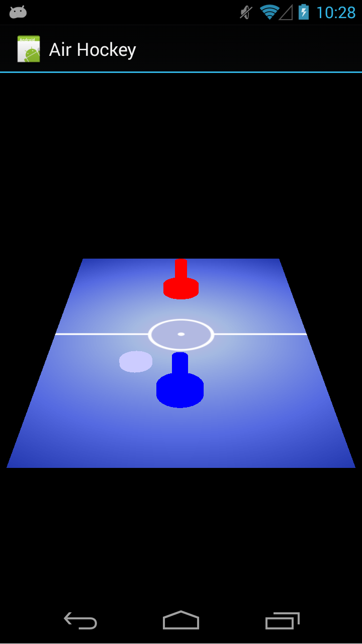
We now have everything in place for Android, and if we run the app, it should look similar to as seen below:

Adding support for iOS

To add support for iOS, we need to update ViewController.m and add support for touch events. To do that and update the frame rate at the same time, let’s add the following to viewDidLoad: before the call to [self setupGL]:

view.userInteractionEnabled = YES;
self.preferredFramesPerSecond = 60;

To listen to the touch events, we need to override a few methods. Let’s add the following methods before - (void)glkView:(GLKView *)view drawInRect:(CGRect)rect:

static CGPoint getNormalizedPoint(UIView* view, CGPoint locationInView)
{
    const float normalizedX = (locationInView.x / view.bounds.size.width) * 2.f - 1.f;
    const float normalizedY = -((locationInView.y / view.bounds.size.height) * 2.f - 1.f);
    return CGPointMake(normalizedX, normalizedY);
}

- (void)touchesBegan:(NSSet *)touches withEvent:(UIEvent *)event
{
    [super touchesBegan:touches withEvent:event];
    UITouch* touchEvent = [touches anyObject];
    CGPoint locationInView = [touchEvent locationInView:self.view];
    CGPoint normalizedPoint = getNormalizedPoint(self.view, locationInView);
    on_touch_press(normalizedPoint.x, normalizedPoint.y);
}

- (void)touchesMoved:(NSSet *)touches withEvent:(UIEvent *)event
{
    [super touchesMoved:touches withEvent:event];
    UITouch* touchEvent = [touches anyObject];
    CGPoint locationInView = [touchEvent locationInView:self.view];
    CGPoint normalizedPoint = getNormalizedPoint(self.view, locationInView);
    on_touch_drag(normalizedPoint.x, normalizedPoint.y);
}

- (void)touchesEnded:(NSSet *)touches withEvent:(UIEvent *)event
{
    [super touchesEnded:touches withEvent:event];
}

- (void)touchesCancelled:(NSSet *)touches withEvent:(UIEvent *)event
{
    [super touchesCancelled:touches withEvent:event];
}

This is similar to the Android code in that it takes the input touch event, converts it to OpenGL’s normalized device coordinate space, and then sends it on to our game code.

Our iOS app should look similar to the following image:

Adding support for emscripten

Adding support for emscripten is just as easy. Let’s first add the following to the top of main.c:

static void handle_input();
// ...
int is_dragging;

At the beginning of do_frame(), add a call to handle_input();:

static void do_frame()
{
	handle_input();
	// ...

Add the following for handle_input:

static void handle_input()
{
	glfwPollEvents();
	const int left_mouse_button_state = glfwGetMouseButton(GLFW_MOUSE_BUTTON_1);
	if (left_mouse_button_state == GLFW_PRESS) {
		int x_pos, y_pos;
		glfwGetMousePos(&x_pos, &y_pos);
		const float normalized_x = ((float)x_pos / (float) width) * 2.f - 1.f;
	    const float normalized_y = -(((float)y_pos / (float) height) * 2.f - 1.f);

		if (is_dragging == 0) {
			is_dragging = 1;
			on_touch_press(normalized_x, normalized_y);
		} else {
			on_touch_drag(normalized_x, normalized_y);
		}
	} else {
		is_dragging = 0;
	}
}

This code sets is_dragging depending on whether we just clicked the primary mouse button or if we’re currently dragging the mouse. Depending on the case, we’ll call either on_touch_press or on_touch_drag. The code to normalize the coordinates is the same as in Android and iOS, and indeed a case could be made to abstract out into the common game code, and just pass in the raw coordinates relative to the view size to that game code.

After compiling with emcc make, we should get output similar to the below:

Exploring further

That concludes our air hockey project! The full source code for this lesson can be found at the GitHub project. You can find a more in-depth look at the concepts behind the project from the perspective of Java Android in OpenGL ES 2 for Android: A Quick-Start Guide. For exploring further, there are many things you could add, like improved graphics, support for sound, a simple AI, multiplayer (on the same device), scoring, or a menu system.

Whether you end up using a commercial cross-platform solution like Unity or Corona, or whether you decide to go the independent route, I hope this series was helpful to you and most importantly, that you enjoy your future projects ahead and have a lot of fun with them. 🙂